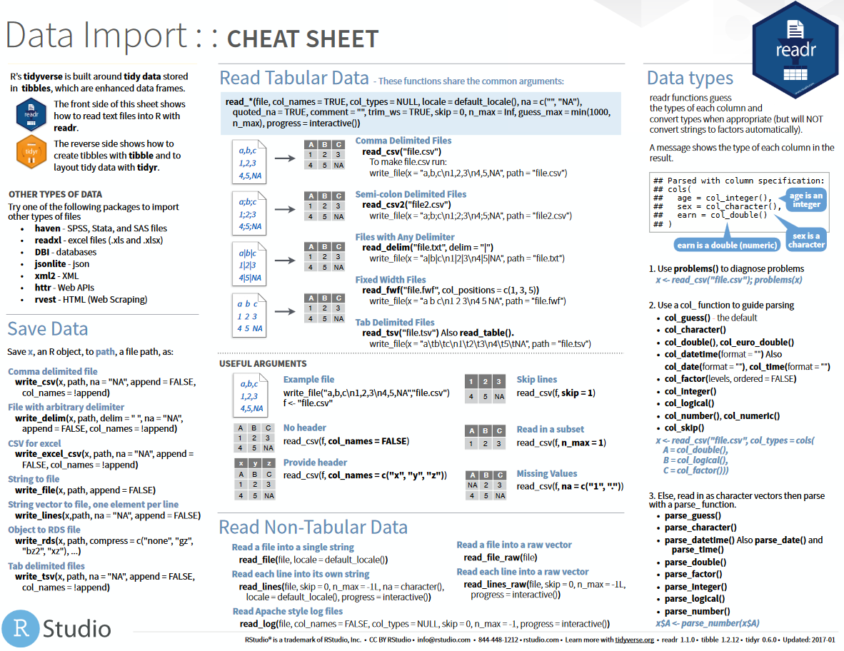
“Tidy datasets are all alike, but every messy dataset is messy in its own way.” - Hadley Wickham
The notes below are modified from the excellent Dataframe Manipulation and freely available on the Software Carpentry website.
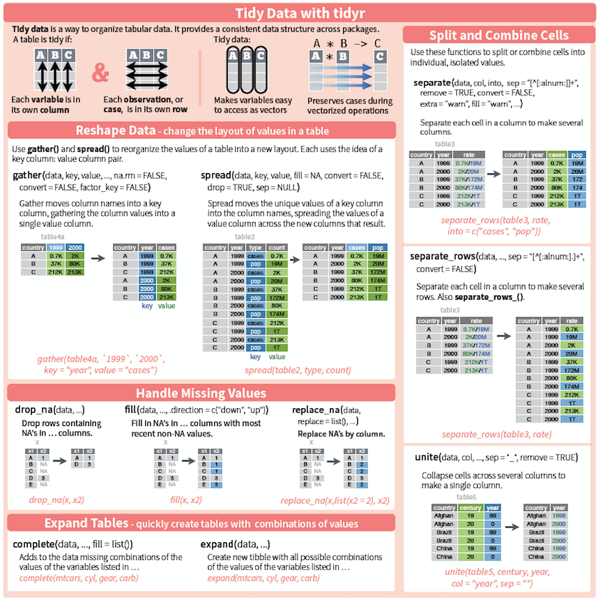
The goal of tidyr is to help you create tidy data. Tidy data is data where: Every column is variable. Every row is an observation. The second page of the new Data Import cheat sheet now contains the details for tidyr. Raw.githubusercontent.com data-import.pdf.
Load the libraries:
In this section, we will learn a consistent way to organize the data in R, called tidy data. Getting the data into this format requires some upfront work, but that work pays off in the long term. Once you have tidy data and the tools provided by the tidyr, dplyr and ggplot2 packages, you will spend much less time munging/wrangling data from one representation to another, allowing you to spend more time on the analytic questions at hand.
Tibble
For now, we will use tibble instead of R’s traditional data.frame. Tibble is a data frame, but they tweak some older behaviors to make life a little easier.
Let’s use Keeling_Data as an example:
You can coerce a data.frame to a tibble using the as_tibble() function:
Tidy dataset
There are three interrelated rules which make a dataset tidy:
- Each variable must have its own column;
- Each observation must have its own row;
- Each value must have its own cell;
These three rules are interrelated because it’s impossible to only satisfy two of the three. That interrelationship leads to an even simpler set of practical instructions:
- Put each dataset in a tibble
- Put each variable in a column
Why ensure that your data is tidy? There are two main advantages:
There’s a general advantage to picking one consistent way of storing data. If you have a consistent data structure, it’s easier to learn the tools that work with it because they have an underlying uniformity. If you ensure that your data is tidy, you’ll spend less time fighting with the tools and more time working on your analysis.
There’s a specific advantage to placing variables in columns because it allows R’s vectorized nature to shine. That makes transforming tidy data feel particularly natural.
tidyr,dplyr, andggplot2are designed to work with tidy data.
The dplyr package provides a number of very useful functions for manipulating dataframes in a way that will reduce the self-repetition, reduce the probability of making errors, and probably even save you some typing. As an added bonus, you might even find the dplyr grammar easier to read.
Here we’re going to cover commonly used functions as well as using pipes %>% to combine them.
Using select()
Use the select() function to keep only the variables (cplumns) you select.
The pipe symbol %>%
Above we used ‘normal’ grammar, but the strengths of dplyr and tidyr lie in combining several functions using pipes. Since the pipes grammar is unlike anything we’ve seen in R before, let’s repeat what we’ve done above using pipes.
x %>% f(y) is the same as f(x, y)
The above lines mean we first call the Keeling_Data_tbl tibble and pass it on, using the pipe symbol%>%, to the next step, which is the select() function. In this case, we don’t specify which data object we use in the select() function since in gets that from the previous pipe. The select() function then takes what it gets from the pipe, in this case the Keeling_Data_tbl tibble, as its first argument. By using pipe, we can take output of the previous step as input for the next one, so that we can avoid defining and calling unnecessary temporary variables. You will start to see the power of pipe later.
Using filter()
Use filter() to get values (rows):
If we now want to move forward with the above tibble, but only with quality 1 , we can combine select() and filter() functions:
You see here we have used the pipe twice, and the scripts become really clean and easy to follow.
Using group_by() and summarize()
Now try to ‘group’ monthly data using the group_by() function, notice how the ouput tibble changes:
The group_by() function is much more exciting in conjunction with the summarize() function. This will allow us to create new variable(s) by using functions that repeat for each of the continent-specific data frames. That is to say, using the group_by() function, we split our original dataframe into multiple pieces, then we can run functions (e.g., mean() or sd()) within summarize().
Here we create a new variable (column) monthly_mean, and append it to the groups (month in this case). Now, we get a so-called monthly climatology.
You can also use arrange() and desc() to sort the data:
Let’s add more statistics to the monthly climatology:
Here we call the n() to get the size of a vector.
Using mutate()

We can also create new variables (columns) using the mutate() function. Here we create a new column co2_ppb by simply scaling co2 by a factor of 1000.
When creating new variables, we can hook this with a logical condition. A simple combination of mutate() and ifelse() facilitates filtering right where it is needed: in the moment of creating something new. This easy-to-read statement is a fast and powerful way of discarding certain data or for updating values depending on this given condition.
Let’s create a new variable co2_new, it is equal to co2 when quality1, otherwise it’s NA:
Combining dplyr and ggplot2
Just as we used %>% to pipe data along a chain of dplyr functions we can use it to pass data to ggplot(). Because %>% replaces the first argument in a function we don’t need to specify the data = argument in the ggplot() function.
By combining dplyr and ggplot2 functions, we can make figures without creating any new variables or modifying the data.
As you will see, this is much easier than what we have done in Section 3. This is the power of a tidy dataset and its related functions!
Let’s plot CO2 of the same month as a function of decimal_date, with the color option:
Or plot the same data but in panels (facets), with the facet_wrap function:
The ‘long’ layout or format is where:
- each column is a variable
- each row is an observation
For the ‘wide’ format, each row is often a site/subject/patient and you have multiple observation variables containing the same type of data. These can be either repeated observations over time, or observation of multiple variables (or a mix of both).
You may find data input may be simpler, or some other applications may prefer the ‘wide’ format. However, many of R’s functions have been designed assuming you have ‘longer’ formatted data.
Here we use tidyr package to efficiently transform the data shape regardless of the original format.
‘Long’ and ‘wide’ layouts mainly affect readability. For humans, the ‘wide’ format is often more intuitive since we can often see more of the data on the screen due to its shape. However, the ‘long’ format is more machine-readable and is closer to the formatting of databases.
Long to wide format with spread()
Spread rows into columns:
Wide to long format with gather()
Gather columns into rows:
Exercise #1
Please go over the notes once again, make sure you understand the scripts.
Exercise #2
Using the tools/functions covered in this section, to solve More about Mauna Loa CO2 in Lab 01.
- R for Data Science, see chapter 10 and 12.
- Data wrangling with R, with a video
- Reshaping data using tidyr package
Previously, we described the essentials of R programming and provided quick start guides for importing data into R as well as converting your data into a tibble data format, which is the best and modern way to work with your data.
[Figure adapted from RStudio data wrangling cheatsheet (see reference section)]
A data set is called tidy when:
- each column represents a variable
- and each row represents an observation
Note that, all column names (except state) have been collapsed into a single key column (here “arrest_attribute”). Their values have been put into a value column (here “arrest_estimate”). Note that, the two columns Murder and Assault have been collapsed and the remaining columns (state, UrbanPop and Rape) have been duplicated. The remaining state column is duplicated. You should use the function gather_() which takes character vectors, containing column names, instead of unquoted column names The simplified syntax is as follow: As an example, type this: Spread “my_data2” to turn back to the original data: You should use the function spread_() which takes strings specifying key and value columns instead of unquoted column names The simplified syntax is as follow: As an example, type this: The R code below uses the data set “my_data” and unites the columns Murder and Assault You should use the function unite_() as follow. As an example, type this: Separate the column “Murder_Assault” [in my_data4] into two columns Murder and Assault: You should use the function separate_() as follow. As an example, type this: It’s possible to combine multiple operations using maggrittr forward-pipe operator : %>%. For example, x %>% f is equivalent to f(x). In the following R code: You should tidy your data for easier data analysis using the R package tidyr, which provides the following functions. Collapse multiple columns together into key-value pairs (long data format): gather(data, key, value, …) Spread key-value pairs into multiple columns (wide data format): spread(data, key, value) Unite multiple columns into one: unite(data, col, …) This analysis has been performed using R (ver. 3.2.3). This section contains best data science and self-development resources to help you on your path.spread(): spread two columns into multiple columns
unite(): Unite multiple columns into one

separate(): separate one column into multiple
Dplyr Cheat Sheet Pdf

Chaining multiple operations
R Dataframe Cheat Sheet
Show me some love with the like buttons below... Thank you and please don't forget to share and comment below!!
Montrez-moi un peu d'amour avec les like ci-dessous ... Merci et n'oubliez pas, s'il vous plaît, de partager et de commenter ci-dessous!Recommended for You!
More books on R and data science Recommended for you
Coursera - Online Courses and Specialization
Data science
Popular Courses Launched in 2020
Tidyverse Cheat Sheet Pdf
Trending Courses
Books - Data Science
Our Books
Others
Want to Learn More on R Programming and Data Science?
Follow us by EmailOn Social Networks:Rstudio Dplyr Cheat Sheet
Click to follow us on Facebook and Google+ :
Comment this article by clicking on 'Discussion' button (top-right position of this page)